Cycle completion
Given a pattern such as A C B A A C B A, Proctor was better at continuing the whole cycle. The CE model tended to collapse onto a single preferred letter. Here, repeating the requested pattern was success, not an unwanted loop.
Project 05 · Reference v1
Training against doom loops
Proctor is an experimental training objective developed to combat doom loops in small language models.
In the original roughly 12-million-parameter experiments, it substantially reduced looping under ordinary sampling settings, despite worsening conventional next-token prediction scores. Predicting held-out text more accurately and producing more useful autoregressive behavior are not necessarily the same outcome.
Read the original account ↗01 / The problem
A doom loop is a generation that gets stuck repeating the same words or phrases. The small CE-trained models in this study tended to enter these loops on almost every prompt.
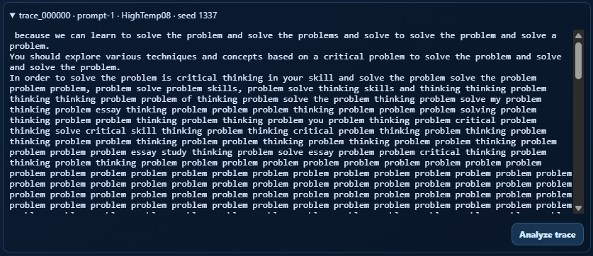
The collapse was often gradual. A response could circle around a few words long before repeating one phrase exactly. In this example, “problem,” “thinking,” and “solve” increasingly dominate, until the generation is almost entirely “problem.”
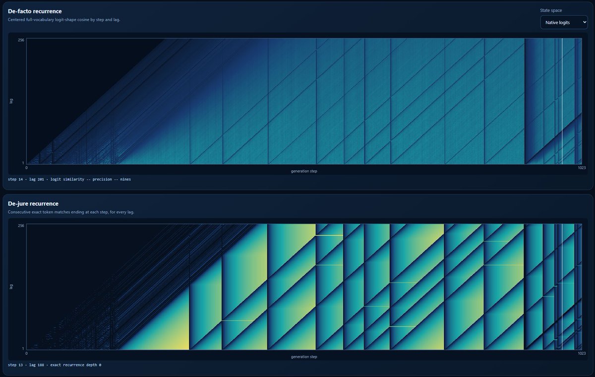
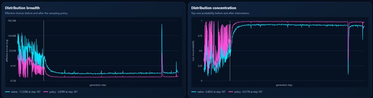
The investigation therefore looked at both the generated tokens and the model's logits—the scores underlying its next-token probabilities. Similar distributions could recur before exact text repetition became obvious. Sampling could delay the visible collapse without removing the underlying pattern.
02 / The idea
The name comes from an exam proctor watching a student repeatedly guess the same multiple-choice answer. A decent score can conceal a shortcut: the student has learned what to guess, not when the answer is appropriate.
The working hypothesis was that small networks can similarly rely too much on easy uncertainty strategies: common connective words, familiar autocomplete continuations, and copying subjects already present in the generation. These strategies may help next-token likelihood while reinforcing a loop during free-running generation.
Proctor makes repeatedly overused wrong alternatives more expensive. Version 1 does not penalize a token's probability at positions where it is correct. Instead, it measures how strongly the model keeps assigning probability to that token where it is wrong.
03 / The objective
Proctor v1 adds a sequence-local concentration penalty to ordinary mean cross-entropy. Its coefficient is fixed at one.
objective = mean_cross_entropy + mean_sequence_penaltyEach item has its own wrong-position denominator. Sequences are not merged before calculating the squared cost. There is no top-k approximation, corpus-frequency table, moving history, detached gradient, or second model evaluation.
Take a four-token vocabulary, with A correct at all three positions and assigned probability 0.50 each time. Put the remaining probabilities at 0.48, 0.01, and 0.01. Always favoring B is the repeated case; rotating the 0.48 through B, C, and D is the distributed case.
| Quantity | Repeated | Distributed |
|---|---|---|
| Mean CE, nats/token | 0.693147 | 0.693147 |
| Proctor penalty | 0.441800 | 0.000000 |
| Combined objective | 1.134947 | 0.693147 |
A is omitted from the pressure statistic because it has no opportunities to be wrong. Equal pressures among B, C, and D have zero penalty; cross-entropy still supplies the incentive to predict A correctly. The included example reproduces the calculation and checks finite gradients.
04 / Observed behavior
The original account describes a roughly 12M dense GPT trained with Proctor while keeping the comparison's data, architecture, context, and vocabulary the same. Under ordinary sampling settings, the Proctor model rarely entered a doom loop where the CE model usually did.
This was the intended result. The model could still ramble, and both models still performed poorly under top-1 generation; Proctor was somewhat less affected. The observed improvement was not a claim that the model had become a broadly capable assistant.
Given a pattern such as A C B A A C B A, Proctor was better at continuing the whole cycle. The CE model tended to collapse onto a single preferred letter. Here, repeating the requested pattern was success, not an unwanted loop.
With a prompt such as Zorb = red, Flerp = blue, Zorb =, Proctor was better at supplying red. These were exploratory probes of very small capabilities, not a general reasoning benchmark.
These behavioral observations are reported in Greed, Doom, and Power. The article does not provide numerical doom-loop incidence rates or scored tables for these probes. The retained measurement package below answers different questions: what happened to held-out likelihood, and to the concentration statistic itself?
05 / Retained measurements
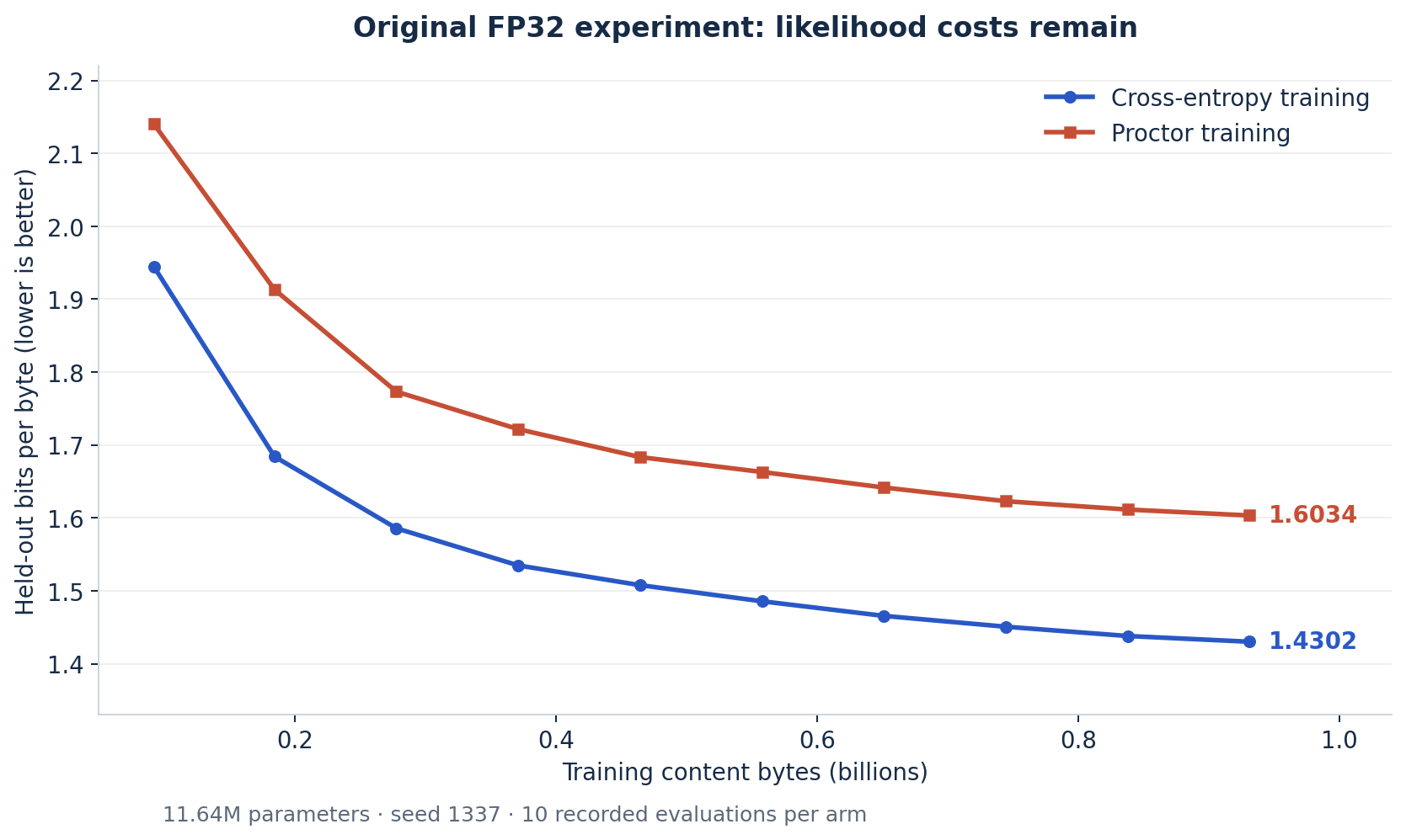
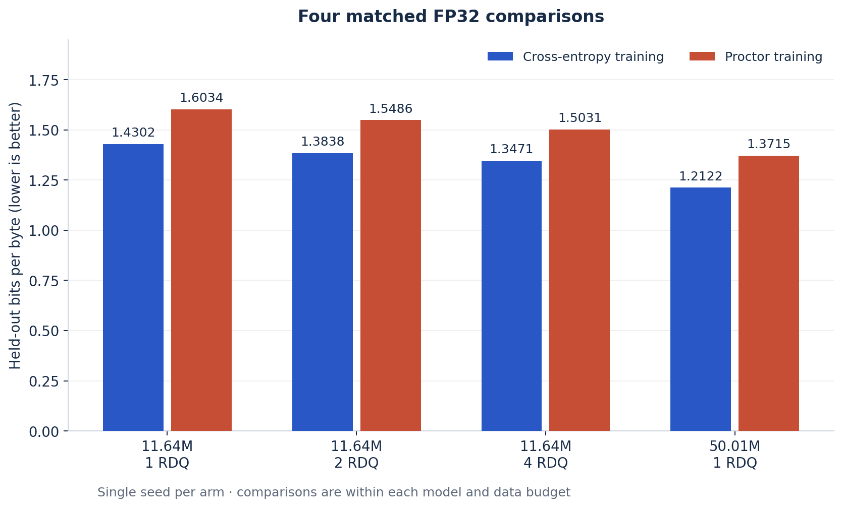
In every reported matched FP32 pair, Proctor had worse held-out bits per byte (BPB). Lower BPB is better: it measures held-out negative log-likelihood in bits per content byte, not generation quality or accuracy.
The original FP32 comparison used 11,637,760 parameters, six layers of width 320, a 12,096-token BPE vocabulary, a 1,152-token context, FineWeb data, fused AdamW, and seed 1337. It ran for 203,920 updates. Within each reported FP32 pair, the recorded initial configurations differ only in objective and output directory.
| Model / budget | CE BPB | Proctor BPB | BPB change |
|---|---|---|---|
| 11.64M · 1 RDQ | 1.4302 | 1.6034 | +12.1% |
| 11.64M · 2 RDQ | 1.3838 | 1.5486 | +11.9% |
| 11.64M · 4 RDQ | 1.3471 | 1.5031 | +11.6% |
| 50.01M · 1 RDQ | 1.2122 | 1.3715 | +13.1% |
The study's budget notation, 1 RDQ, means 80 raw content bytes per trainable parameter. It does not mean equal training bytes across model sizes. Each row is a within-pair comparison, with one recorded seed per arm; the larger model also has a different tokenizer.
The historical TF32 pair has full-validation concentration scores: mean sequence penalty fell from 4.055883 to 0.296039, a 92.7% reduction. BPB rose from 1.429681 to 1.609593, or 12.6%. That percentage reduction belongs to this TF32 pair—not to the FP32 comparisons above, and not to a measured doom-loop rate.
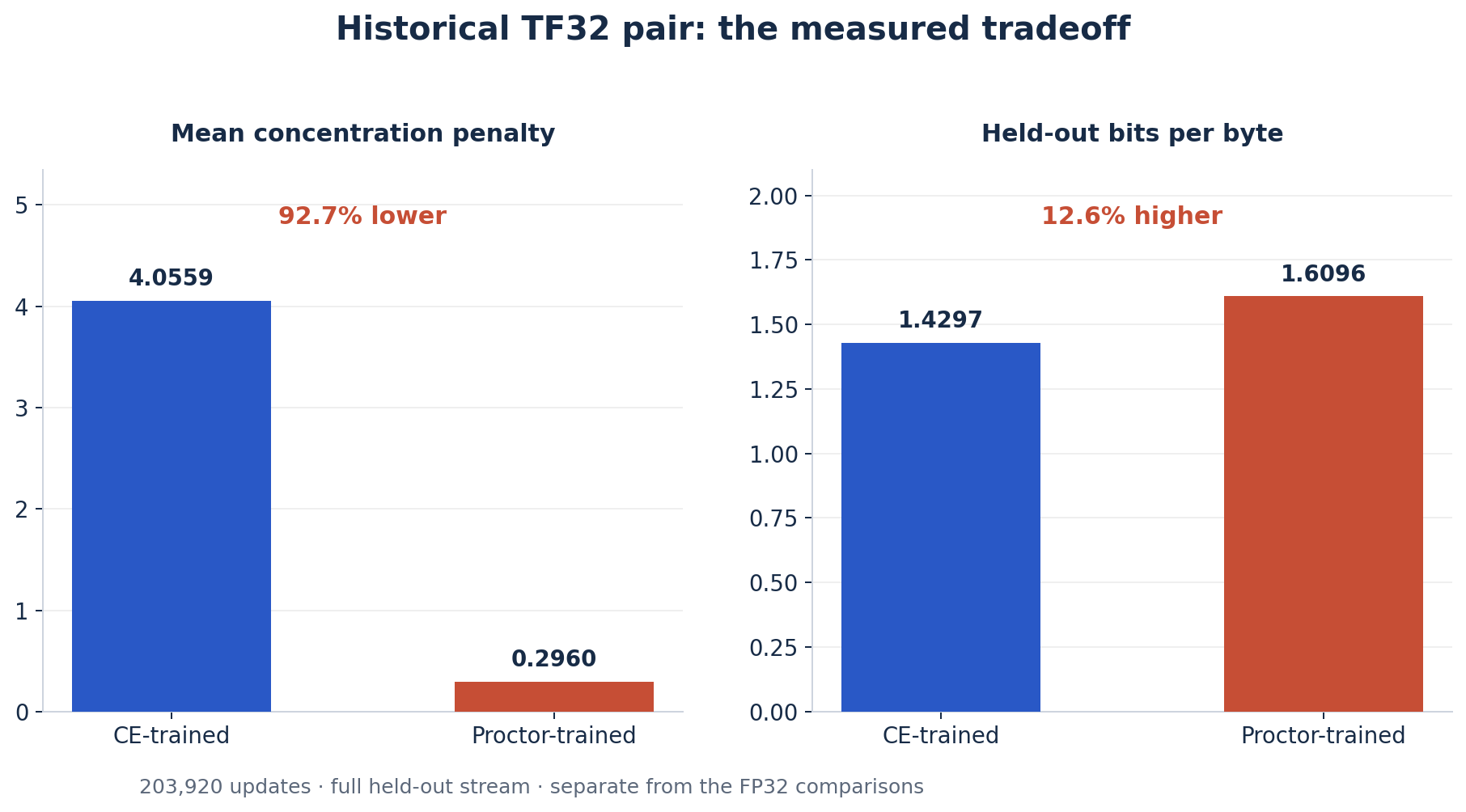
The historical TF32 arms have different dataset-wrapper and architecture labels, but matching physical validation-token and byte-length hashes, model dimensions, and checkpoint steps. Their scoring summaries report float32 tensor dtype without independently recording evaluation matmul mode. No full-validation concentration summaries were found for the inspected FP32 pairs. The package preserves the corrected historical precision labels and the underlying records.
06 / Reference v1
A portable PyTorch loss, a runnable numerical example, tests, the explainer, and retained experiment evidence. Python 3.10+ and PyTorch; CPU is sufficient for the example and tests.
The reference accepts complete, equal-length, unpadded sequences and aligned targets. It computes in float32, with no padding masks or ignored targets. Sequence boundaries, vocabulary, and length affect the penalty; changes to these choices define a different variant.
The archive does not include the original corpus, tokenizer, trained weights, or full training system. It reproduces the objective, not the complete historical training experiments. It makes no throughput claim.